1. 频率分析 (1):从 fchk 文件得到分子频率与简正模式#
创建时间:2019-10-04;最后修改:2021-06-21
在这份文档中,我们将简单地讨论从 Gaussian 生成的 formated checkpoint 文件 (fchk 或 fch 后缀名),依据分子的 Hessian 矩阵,给出分子的振动频率与其对应的简正运动模式。
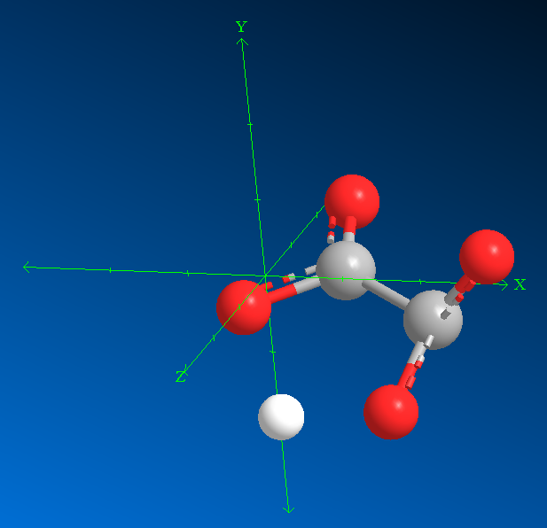
我们所计算的分子是以下显然没有优化到能量最低结构的 C2O4H+ 分子。之所以选择这样一个分子,是因为作者希望能正确地计算出虚频。
警告
不处于能量最低结构的分子一般来说不适合用作频率分析。此时绘制的分子光谱图从理论上是与不可能与实验相符的。
这份文档尽管使用了有虚频的分子,但若要进行真正的光谱绘制,仍然需要先对分子的结构进行优化。
警告
这篇文档以后有可能会作一定程度的修改。有兴趣的读者也应当参考 Gaussian 白皮书 Vibrational Analysis in Gaussian。
分子结构如下:
from IPython.display import Image
Image(filename="assets/mol_fig.PNG", width=250)
分子对应的输入卡 C2O4H.gjf、输出文件 C2O4H.out 与 fchk 文件 C2O4H.fchk 在链接中可供下载。这份文档的目标将是重复输出文件中的分子频率 Frequencies (单位 cm-1) 与简正坐标部分;而下一份文档将会重复红外强度 IR Inten (单位 km/mol) 与绘制红外光谱。以下是其中一部分频率分析的输出:
with open("C2O4H.out", "r") as f:
    while "and normal coordinates" not in f.readline(): continue
    for _ in range(17): print(f.readline()[:-1])
                     1                      2                      3
                     A                      A                      A
 Frequencies -- -3561.4012             -2816.7847              -111.1073
 Red. masses --     6.8911                 1.1249                14.6979
 Frc consts  --    51.4966                 5.2586                 0.1069
 IR Inten    --  9128.2276              4124.7910                 5.3095
 Raman Activ -- 90326.7283              3896.5620                15.3400
 Depolar (P) --     0.7167                 0.2640                 0.5287
 Depolar (U) --     0.8350                 0.4177                 0.6917
  Atom  AN      X      Y      Z        X      Y      Z        X      Y      Z
     1   6     0.54  -0.07  -0.05     0.04  -0.01   0.03    -0.02   0.16   0.01
     2   8    -0.14   0.02   0.01    -0.03   0.03  -0.03     0.03   0.42   0.26
     3   6    -0.28   0.10  -0.25    -0.04   0.02  -0.03    -0.01   0.10  -0.04
     4   8     0.03  -0.04   0.08    -0.02  -0.01   0.02     0.10  -0.33  -0.34
     5   8    -0.12  -0.03   0.09    -0.01   0.01  -0.02     0.04  -0.46  -0.20
     6   8     0.08   0.03   0.05     0.00  -0.01   0.01    -0.14   0.19   0.31
     7   1    -0.67  -0.18  -0.08     0.88  -0.32   0.33     0.01  -0.21  -0.18
备注
频率分析 (1) 文档的目的与卢天 (Sobereva) 的 Hess2freq 程序 [1] 的程序基本相同,文档的编写过程也受到不少启发。
但另一方面,这份文档将会解决投影整体平动和转动模式。因此,这份文档原则上应当能通过 Hessian 矩阵,给出更为接近 Gaussian 所输出的频率的结果。而任何量化软件通常都可以计算杂化 GGA 泛函级别的 Hessian,因此这份文档可以用于补足一些不进行频率分析的软件。
这份文档的一个问题会是无法对直线型或说 \(3N-5\) 型分子作频率分析。文档中 \(3N-6\) 的 \(6\) 是 hardcoded 到代码中的。
备注
这篇文档不使用 Einstein Summation Convention。
注意
事实上,作者并不完全理解整个计算过程的原理;但这似乎是个可行的方案。
1.1. 环境准备#
下述引入的包中,
FormchkInterface可以用来读取 fchk 文件的信息;文件出自 pyxdh 项目。文档中我们可能会使用众多物理常数。这些由 SciPy 提供,数据来源是 CODATA 2014。
from formchk_interface import FormchkInterface
import numpy as np
from functools import partial
import scipy

np.set_printoptions(5, linewidth=150, suppress=True)
np.einsum = partial(np.einsum, optimize=["greedy", 1024 ** 3 * 2 / 8])
# https://docs.scipy.org/doc/scipy/reference/constants.html
from scipy.constants import physical_constants

E_h = physical_constants["Hartree energy"][0]
a_0 = physical_constants["Bohr radius"][0]
N_A = physical_constants["Avogadro constant"][0]
c_0 = physical_constants["speed of light in vacuum"][0]
e_c = physical_constants["elementary charge"][0]
e_0 = physical_constants["electric constant"][0]
mu_0 = physical_constants["mag. constant"][0]
现在我们准备分子的数据:
natm原子数量 \(n_\mathrm{Atom}\)mol_weight原子质量 \(w_A\),向量长度 \((n_\mathrm{Atom},)\),单位 amumol_coord原子坐标 \(A_t\),矩阵大小 \((n_\mathrm{Atom}, 3)\),单位 Bohrmol_hess坐标二阶梯度 (Hessian 矩阵) \(E_\mathrm{tot}^{A_t B_s}\),张量大小 \((n_\mathrm{Atom}, 3, n_\mathrm{Atom}, 3)\),单位 Eh Bohr-2
本文档中,\(A, B\) 指代原子,\(t, s\) 指代坐标分量 \(x, y\) 或 \(z\)。
fchk = FormchkInterface("C2O4H.fchk")
mol_weight = fchk.key_to_value("Real atomic weights")
natm = mol_weight.size
mol_coord = fchk.key_to_value("Current cartesian coordinates").reshape((natm, 3))
mol_hess = fchk.hessian()
mol_hess = (mol_hess + mol_hess.T) / 2
mol_hess = mol_hess.reshape((natm, 3, natm, 3))
1.2. 包含平动、转动的频率#
这里按照 Hess2freq 程序的思路进行叙述。我们首先生成带原子质量权重的力常数张量 theta
但为了程序便利,我们重定义 theta 的维度信息为 \((3 n_\mathrm{Atom}, 3 n_\mathrm{Atom})\);单位是 Eh Bohr-2 amu-1。
theta = np.einsum("AtBs, A, B -> AtBs", mol_hess, 1 / np.sqrt(mol_weight), 1 / np.sqrt(mol_weight)).reshape(3 * natm, 3 * natm)
随后,我们对其进行对角化,可以立即得到原始的分子频率 e 与简正坐标 q,且维度分别是 \((3 n_\mathrm{Atom}, 3 n_\mathrm{Atom})\) 与 \((3 n_\mathrm{Atom},)\)。注意到 e 的单位是 Eh Bohr-2 amu-1,而 q 现在是无量纲量。
e, q = np.linalg.eigh(theta)
现在获得的原始分子频率事实上是力常数除以质量的结果,或者按照 Levine (7ed) p63, eq (4.23) 的表达,为 \(k/m\)。因此,化为以波数表示的频率 freq_cm_1 的公式是
其中,\(c_0\) 表示真空光速。在实行具体计算前,需要将单位转换为国际单位制。最终会将频率转成 cm-1 单位。
freq_cm_1 = np.sqrt(np.abs(e * E_h * 1000 * N_A / a_0**2)) / (2 * np.pi * c_0 * 100) * ((e > 0) * 2 - 1)
freq_cm_1
array([-3561.40505, -2816.91767,  -168.16445,  -156.49378,  -118.3671 ,    -0.05708,     0.00635,     0.02696,    43.3215 ,   289.57484,   359.82004,
         542.70646,   584.63229,   646.04288,   680.41788,   775.32894,  1115.58713,  1346.89468,  1521.52455,  1593.04881,  1969.81362])
需要留意,复数的频率实际上是虚数频率,或者说是现实中不存在的频率;使用复数表示这些频率仅仅是为了程序方便,以及约定俗称的原因。
由于分子的振动自由度 (对于非线性分子) 是 \(3 n_\mathrm{Atom} - 6\),因此其中有 6 个频率不应当归属于振动频率中。大多数情况下,舍去绝对值最小的六个频率即可;但其值仍然会与 Gaussian 给出的结果有少许的不同。
简正坐标在这里我们暂时不进行更多说明;在叙述去除平动、转动的频率后,我们再讨论简正坐标的导出。
1.3. 去除平动、转动的频率#
去除平动、转动对频率的贡献,其过程大致是预先将平动、转动的模式求取,随后将力常数张量投影到平动、转动模式的补空间 (\(3 n_\mathrm{Atom} - 6\) 维度空间),得到新的力常数张量。
其中的大部分内容应当在 Wilson et al. [2] 的 Chapter 2 可以找到。
1.3.1. 质心坐标#
center_coord \(C_t\) 表示质心坐标,维度 \((3,)\),单位 Bohr。
center_coord = (mol_coord * mol_weight[:, None]).sum(axis=0) / mol_weight.sum()
center_coord
array([ 2.56385, -0.44307, -0.07436])
centered_coord \(A^\mathrm{C}_t\) 是将质心平移至原点后的原子坐标,维度 \((n_\mathrm{Atom}, 3)\),单位 Bohr。
centered_coord = mol_coord - center_coord
1.3.2. 转动惯量本征向量#
rot_tmp \(I_{ts}\) 是转动惯量相关的矩阵,在初始化时维度为 \((n_\mathrm{Atom}, 3, 3)\),最终结果通过求和得到 \((3, 3)\) 的矩阵,单位 Bohr2 amu。
rot_tmp = np.zeros((natm, 3, 3))
rot_tmp[:, 0, 0] = centered_coord[:, 1]**2 + centered_coord[:, 2]**2
rot_tmp[:, 1, 1] = centered_coord[:, 2]**2 + centered_coord[:, 0]**2
rot_tmp[:, 2, 2] = centered_coord[:, 0]**2 + centered_coord[:, 1]**2
rot_tmp[:, 0, 1] = rot_tmp[:, 1, 0] = - centered_coord[:, 0] * centered_coord[:, 1]
rot_tmp[:, 1, 2] = rot_tmp[:, 2, 1] = - centered_coord[:, 1] * centered_coord[:, 2]
rot_tmp[:, 2, 0] = rot_tmp[:, 0, 2] = - centered_coord[:, 2] * centered_coord[:, 0]
rot_tmp = (rot_tmp * mol_weight[:, None, None]).sum(axis=0)
rot_eig \(R_{ts}\) 是转动惯量相关的对称矩阵 \(I_{ts}\) 所求得的本征向量,维度 \((3, 3)\),无量纲。
_, rot_eig = np.linalg.eigh(rot_tmp)
rot_eig
array([[ 0.80658, -0.54971,  0.21739],
       [-0.16056, -0.55765, -0.8144 ],
       [ 0.56891,  0.62197, -0.53805]])
1.3.3. 平动、转动投影矩阵#
proj_scr \(P_{A_t q}\) 是平动、转动的 \((3 n_\mathrm{Atom}, 6)\) 维度投影矩阵,其目的是将 \(\Theta^{A_t B_s}\) 中不应对分子振动产生贡献的部分投影消去,剩余的 \(3 n_\mathrm{Atom} - 6\) 子空间用于求取实际的分子振动频率。但在初始化 proj_scr \(P_{A_t q}\) 时,先使用 \((n_\mathrm{Atom}, 3, 6)\) 维度的张量。
在计算投影矩阵前,我们先生成 rot_coord \(\mathscr{R}_{Asrw}\) 转动投影相关量,维度 \((n_\mathrm{Atom}, 3, 3, 3)\):
rot_coord = np.einsum("At, ts, rw -> Asrw", centered_coord, rot_eig, rot_eig)
rot_coord.shape
(7, 3, 3, 3)
随后我们给出 proj_scr 的计算表达式。proj_scr 的前三列表示平动投影,当 \(q \in (x, y, z) = (0, 1, 2)\) 时,
而当 \(q \in (x, y, z) = (3, 4, 5)\) 时,
最终,我们会将 \(P_{A_t q}\) 中关于 \(A_t\) 的维度进行归一化,因此最终获得的 \(P_{A_t q}\) 是无量纲的。
proj_scr = np.zeros((natm, 3, 6))
proj_scr[:, (0, 1, 2), (0, 1, 2)] = 1
proj_scr[:, :, 3] = (rot_coord[:, 1, :, 2] - rot_coord[:, 2, :, 1])
proj_scr[:, :, 4] = (rot_coord[:, 2, :, 0] - rot_coord[:, 0, :, 2])
proj_scr[:, :, 5] = (rot_coord[:, 0, :, 1] - rot_coord[:, 1, :, 0])
proj_scr *= np.sqrt(mol_weight)[:, None, None]
proj_scr.shape = (-1, 6)
proj_scr /= np.linalg.norm(proj_scr, axis=0)
proj_scr
array([[ 0.36722,  0.     ,  0.     ,  0.00369,  0.05794,  0.11255],
       [ 0.     ,  0.36722,  0.     ,  0.04243, -0.17071,  0.09139],
       [ 0.     ,  0.     ,  0.36722,  0.00675, -0.10185, -0.09286],
       [ 0.42396,  0.     ,  0.     ,  0.01229, -0.02015, -0.0705 ],
       [ 0.     ,  0.42396,  0.     , -0.49194, -0.29189,  0.22557],
       [ 0.     ,  0.     ,  0.42396, -0.15626, -0.27952, -0.36992],
       [ 0.36722,  0.     ,  0.     ,  0.03114,  0.00301, -0.06566],
       [ 0.     ,  0.36722,  0.     ,  0.11694,  0.18118, -0.11688],
       [ 0.     ,  0.     ,  0.36722, -0.01115,  0.16511,  0.15039],
       [ 0.42396,  0.     ,  0.     ,  0.16731, -0.02119, -0.43088],
       [ 0.     ,  0.42396,  0.     , -0.30661,  0.34319, -0.15655],
       [ 0.     ,  0.     ,  0.42396, -0.32374,  0.28897,  0.06287],
       [ 0.42396,  0.     ,  0.     , -0.02565,  0.18716,  0.45037],
       [ 0.     ,  0.42396,  0.     ,  0.3913 , -0.45793,  0.21108],
       [ 0.     ,  0.     ,  0.42396,  0.1468 , -0.24516, -0.13753],
       [ 0.42396,  0.     ,  0.     , -0.19609, -0.19816,  0.03903],
       [ 0.     ,  0.42396,  0.     ,  0.31205,  0.3942 , -0.26137],
       [ 0.     ,  0.     ,  0.42396,  0.36608,  0.17829,  0.41139],
       [ 0.10642,  0.     ,  0.     ,  0.04773, -0.00179, -0.11404],
       [ 0.     ,  0.10642,  0.     , -0.17067,  0.01343,  0.01336],
       [ 0.     ,  0.     ,  0.10642, -0.11584,  0.01045, -0.06629]])
最后我们声明,在经过上述投影后的力常数矩阵几乎表现为零:
proj_scr.T @ theta @ proj_scr
array([[-0.     ,  0.     ,  0.     , -0.     , -0.     ,  0.     ],
       [ 0.     ,  0.     ,  0.     , -0.     , -0.     , -0.     ],
       [ 0.     ,  0.     ,  0.     ,  0.     ,  0.     ,  0.     ],
       [-0.     , -0.     ,  0.     , -0.00034,  0.00053, -0.00012],
       [-0.     , -0.     ,  0.     ,  0.00053,  0.00001,  0.00011],
       [ 0.     , -0.     ,  0.     , -0.00012,  0.00011, -0.00021]])
对上述矩阵进行对角化所给出的平动、转动频率如下:
e_tr, _ = np.linalg.eigh(proj_scr.T @ theta @ proj_scr)
np.sqrt(np.abs(e_tr * E_h * 1000 * N_A / a_0**2)) / (2 * np.pi * c_0 * 100) * ((e_tr > 0) * 2 - 1)
array([-142.94819, -65.35067, -0.05708, 0.00635, 0.02696, 102.63548])
1.3.4. 平动、转动投影矩阵的补空间#
既然我们已经得到了平动、转动的投影,那么根据矩阵的原理,相应地我们也能获得其补空间的投影。我们令 proj_inv \(Q_{A_t q}\) 为 \(P_{A_t q}\) 的补空间投影。获得补空间的大致方式是预先定义一个仅有一个分量为 \(1\) 的 \((3 n_\mathrm{Atom}, )\) 维度向量,随后通过 Schmit 正交的方式给出已有投影空间的补空间向量。组合这些 Schmit 正交的向量便获得了 \(Q_{A_t q}\)。
\(Q_{A_t q}\) 的维度本应当是 \((3 n_\mathrm{Atom}, 3 n_\mathrm{Atom} - 6)\) 维。但为了程序编写方便,我们先规定 proj_inv 是 \((3 n_\mathrm{Atom}, 3 n_\mathrm{Atom})\) 维度,并且其中的前 6 列填入 \(P_{A_t q}\);在进行 Schmit 正交化后,再将前 6 列剔除。
proj_inv = np.zeros((natm * 3, natm * 3))
proj_inv[:, :6] = proj_scr
cur = 6
for i in range(0, natm * 3):
    vec_i = np.einsum("Ai, i -> A", proj_inv[:, :cur], proj_inv[i, :cur])
    vec_i[i] -= 1
    if np.linalg.norm(vec_i) > 1e-8:
        proj_inv[:, cur] = vec_i / np.linalg.norm(vec_i)
        cur += 1
    if cur >= natm * 3:
        break
proj_inv = proj_inv[:, 6:]
我们最后获得的 \(Q_{A_t q}\) 是列正交切归一的矩阵,且形式大致是下三角矩阵。但需要留意,对于当前的分子,最后一列只有 6 个非零值,与倒数第二列非零值的数量相差 2 个。
proj_inv[:, :8]
array([[-0.92147, -0.     ,  0.     , -0.     , -0.     ,  0.     , -0.     , -0.     ],
       [ 0.0006 , -0.90876,  0.     ,  0.     ,  0.     , -0.     ,  0.     , -0.     ],
       [-0.01772,  0.0101 , -0.91962,  0.     ,  0.     ,  0.     ,  0.     , -0.     ],
       [ 0.15913, -0.00263,  0.00635, -0.88846,  0.     ,  0.     , -0.     , -0.     ],
       [ 0.00723,  0.22587,  0.00828, -0.0174 , -0.62508, -0.     ,  0.     ,  0.     ],
       [-0.06338,  0.00797,  0.23777,  0.02386,  0.12464, -0.71004, -0.     ,  0.     ],
       [ 0.13864, -0.00562,  0.00379,  0.20568, -0.05571,  0.01213, -0.89165, -0.     ],
       [-0.00242,  0.10806, -0.00617,  0.00599,  0.06901, -0.02449,  0.00896, -0.88757],
       [ 0.02871, -0.01639,  0.11235, -0.00984, -0.01789,  0.10978, -0.00552,  0.00503],
       [ 0.11566, -0.03146,  0.04451,  0.26042, -0.29396,  0.15738,  0.31106,  0.0477 ],
       [ 0.00123,  0.07679, -0.02363,  0.00022,  0.33955,  0.06639, -0.01868,  0.25957],
       [ 0.02455, -0.06306,  0.1274 , -0.01053,  0.12201,  0.23871, -0.01701,  0.00208],
       [ 0.23563,  0.00909, -0.07083,  0.20364,  0.09472, -0.32385,  0.2141 , -0.00369],
       [-0.00144,  0.29684,  0.03556, -0.00183,  0.37737,  0.06574, -0.02848,  0.16881],
       [-0.03163,  0.03906,  0.21245,  0.01424, -0.03451,  0.45782,  0.02184, -0.02423],
       [ 0.16048,  0.0321 ,  0.01383,  0.22974,  0.26819,  0.14629,  0.22725, -0.04739],
       [-0.00589,  0.08555, -0.01393,  0.01471, -0.20618, -0.12656,  0.04452,  0.32995],
       [ 0.06292,  0.02501,  0.10976, -0.01965, -0.21114, -0.11824,  0.00024,  0.01928],
       [ 0.02856, -0.00888,  0.01142,  0.06576, -0.08244,  0.03852,  0.07928,  0.01347],
       [ 0.00179,  0.03386, -0.00375, -0.00353,  0.21735,  0.06231, -0.0204 ,  0.04162],
       [-0.0079 , -0.01404,  0.04718,  0.00238,  0.05775,  0.14602, -0.00114, -0.00595]])
proj_inv[:, 8:]
array([[-0.     , -0.     ,  0.     ,  0.     , -0.     ,  0.     , -0.     ],
       [ 0.     , -0.     ,  0.     ,  0.     ,  0.     , -0.     , -0.     ],
       [ 0.     ,  0.     , -0.     ,  0.     , -0.     , -0.     , -0.     ],
       [ 0.     ,  0.     , -0.     , -0.     ,  0.     , -0.     ,  0.     ],
       [-0.     ,  0.     ,  0.     ,  0.     ,  0.     ,  0.     ,  0.     ],
       [-0.     , -0.     , -0.     , -0.     ,  0.     ,  0.     , -0.     ],
       [ 0.     , -0.     ,  0.     ,  0.     , -0.     ,  0.     , -0.     ],
       [-0.     , -0.     , -0.     , -0.     , -0.     , -0.     , -0.     ],
       [-0.88821,  0.     , -0.     , -0.     , -0.     ,  0.     ,  0.     ],
       [-0.04822, -0.55628,  0.     ,  0.     , -0.     ,  0.     , -0.     ],
       [ 0.03972, -0.14218, -0.60686, -0.     , -0.     ,  0.     , -0.     ],
       [ 0.28906, -0.17446,  0.45345, -0.46401, -0.     ,  0.     ,  0.     ],
       [ 0.06431,  0.06973,  0.00436,  0.05117, -0.55525,  0.     , -0.     ],
       [-0.05364, -0.22108,  0.16095, -0.21835, -0.04109, -0.14297, -0.     ],
       [ 0.18656,  0.31662, -0.22295,  0.16951, -0.42471,  0.25709,  0.     ],
       [-0.01297,  0.40547,  0.02383,  0.0214 ,  0.5487 ,  0.10936, -0.18819],
       [ 0.01152,  0.40633,  0.35634,  0.05943,  0.02677,  0.08518, -0.13536],
       [ 0.27891, -0.14836, -0.26106,  0.18737,  0.44457, -0.05496,  0.07441],
       [-0.01243,  0.32303, -0.11228, -0.28913,  0.02613, -0.43568,  0.74973],
       [ 0.00958, -0.17158,  0.35684,  0.63313,  0.05705,  0.23023,  0.53923],
       [ 0.05897,  0.02469,  0.12176,  0.42675, -0.07912, -0.80524, -0.29643]])
1.3.5. 去除平动、转动部分的频率#
我们将对矩阵 \(\mathbf{Q}^\dagger \mathbf{\Theta} \mathbf{Q}\) 进行对角化;且获得的第 \(q\) 个简正坐标的频率相关量 e \(K_q = k_q / m_q\) 与原始简正坐标 q \(\mathbf{q}^\mathrm{orig}\) 表示如下:
e, q = np.linalg.eigh(proj_inv.T @ theta @ proj_inv)
由此,我们就可以立即获得去除平动、转动部分的,以 cm-1 为单位的,总数为 \(3 n_\mathrm{Atom} - 6\) 的分子频率 freq_cm_1:
freq_cm_1 = np.sqrt(np.abs(e * E_h * 1000 * N_A / a_0**2)) / (2 * np.pi * c_0 * 100) * ((e > 0) * 2 - 1)
freq_cm_1
array([-3561.40117, -2816.7847 ,  -111.10727,   285.51964,   354.79005,   541.46285,   583.67422,   641.59573,   678.70706,   774.75315,  1114.8334 ,
        1341.17965,  1521.15243,  1592.00939,  1969.72731])
1.3.6. 归一化的简正坐标#
方才通过对角化,我们获得的原始简正坐标 q 的维度是 \(3 n_\mathrm{Atom} - 6\)。我们需要通过 q \(\mathbf{q}^\mathrm{orig}\) 重塑回正常的简正坐标的维度 \(q_{A_t q}\) \((3 n_\mathrm{Atom}, 3 n_\mathrm{Atom} - 6)\)。
我们首先给出未经过归一化的简正坐标,命名为 q_unnormed \(q_{A_t q}^\mathrm{unnorm}\),其单位是 amu-1/2。该量将会用于后续的红外强度计算上。其计算过程大致是
q_unnormed = np.einsum("AtQ, A -> AtQ", (proj_inv @ q).reshape(natm, 3, (proj_inv @ q).shape[-1]), 1 / np.sqrt(mol_weight))
q_unnormed = q_unnormed.reshape(-1, q_unnormed.shape[-1])
而将每一个简正坐标的振动强度归一化的矩阵称为 q_normed \(q_{A_t q}\);它是我们的目标的简正坐标。
q_normed = q_unnormed / np.linalg.norm(q_unnormed, axis=0)
我们可以以下述代码核对前三个简正坐标。这些坐标应当与 Gaussian 所输出的坐标几乎相同,或刚好相差正负号。
q_normed.reshape(natm, 3, 3 * natm - 6)[:, :, :3].transpose((2, 0, 1))
array([[[ 0.54001, -0.07088, -0.04608],
        [-0.14273,  0.02387,  0.00516],
        [-0.284  ,  0.09918, -0.24533],
        [ 0.03237, -0.03565,  0.07878],
        [-0.12144, -0.02845,  0.08535],
        [ 0.08194,  0.03046,  0.05426],
        [-0.66966, -0.18195, -0.07812]],

       [[ 0.0408 , -0.01485,  0.03176],
        [-0.02602,  0.02747, -0.02887],
        [-0.03581,  0.01862, -0.02587],
        [-0.02413, -0.01192,  0.01877],
        [-0.01187,  0.00732, -0.02008],
        [ 0.0026 , -0.0054 ,  0.00522],
        [ 0.88356, -0.32216,  0.32609]],

       [[-0.02081,  0.165  ,  0.00726],
        [ 0.02702,  0.41713,  0.26319],
        [-0.01085,  0.09639, -0.03556],
        [ 0.09566, -0.32921, -0.34068],
        [ 0.03741, -0.46378, -0.19918],
        [-0.13693,  0.19313,  0.30902],
        [ 0.00955, -0.21243, -0.17633]]])
1.4. 修订记录#
2021-06-21:重新写了 Schmidt 正交化代码。我不太理解当时的代码到底为什么是对的 (>.<)